Fractals

Fractals are infinitely complex patterns that gain shape from simple structures bound to various mathematical rules and constraints. They are useful in modelling structures (such as snowflakes) in which similar patterns recur at progressively smaller scales, and in describing partly random or chaotic phenomena such as crystal growth and galaxy formation. They act as to bridge to explain naturally occurring shapes over a set of fixed rules. Over this article, I have explored few of the fascinating fractals I have come across and the visual treat they offer.

Lindenmayer Systems

An L-system consists of an alphabet of symbols that can be used to make strings, a collection of production that expand each symbol into some larger string of symbols, an initial “axiom” string from which to begin construction, and a mechanism for translating the generated strings into geometric structures.

The L-Systems over controlled iterations provide us an unique string with perceived geometric properties. This motion is perceived using turtle graphics where the turtle moves with commands that are relative to its own position, such as “move forward 10 spaces” and “turn left 90 degrees” depending upon each variable in the string. The pen carried by the turtle can also be controlled, by enabling it, setting its colour, or setting its width.

Some of the constant literals of Lindenmayer Systems.

X → F+[[X]-X]-F[-FX]+X

• F means “draw forward”

• − means “turn left by some angle”

• • means “turn right some angle”.

• X and Y mostly does not correspond to any drawing action and is used to control the evolution of the curve.

• The square bracket “[“ corresponds to saving the current values for position and angle, which are restored when the corresponding “]” is executed.

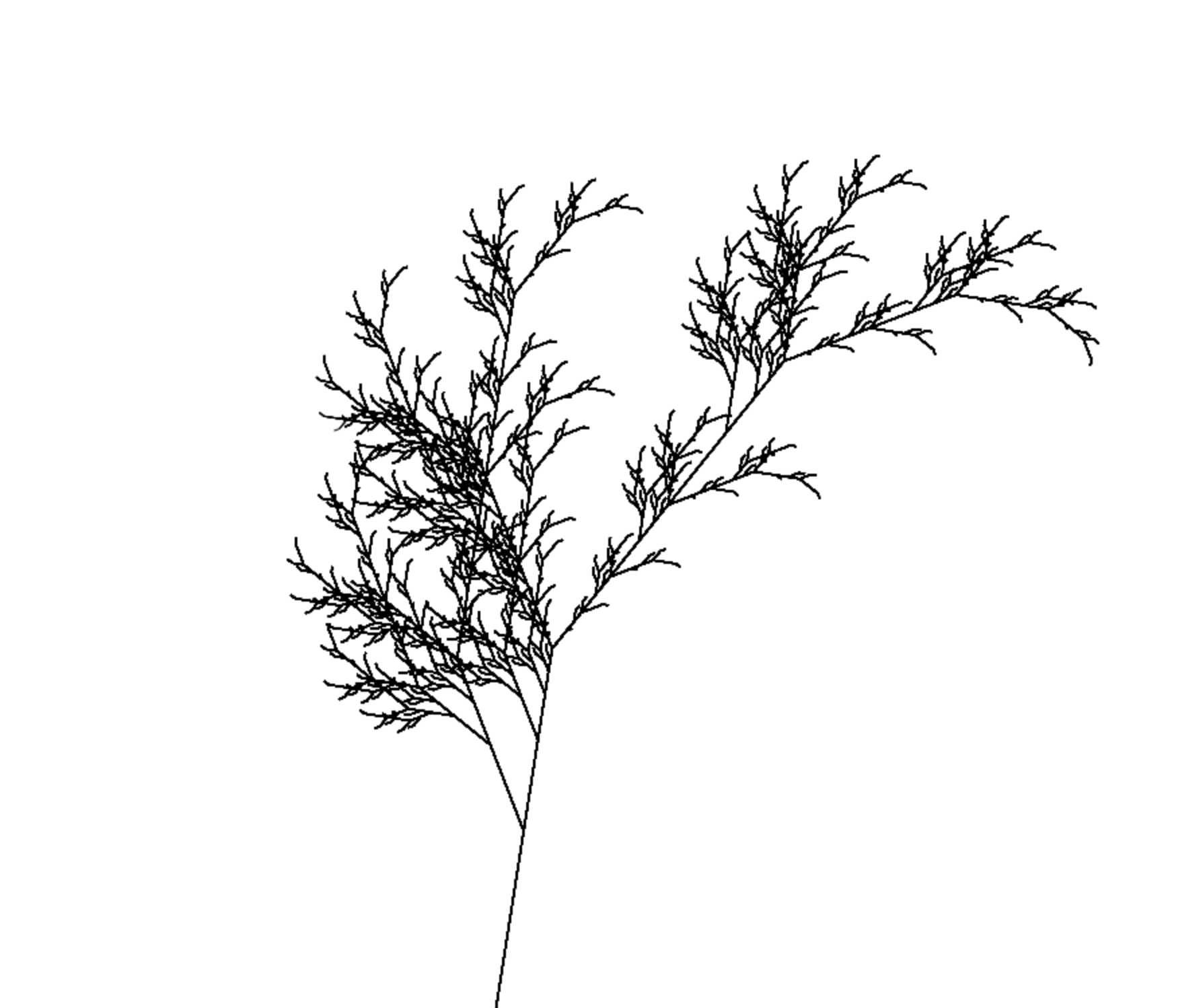
Fractal Plant

**variables** : X F
**constants** : + − [ ]
**start** : X
**rules** : (X → F+[[X]-X]-F[-FX]+X), (F → FF)
**angle** : 30°

Under 7 iterations, it produces this beautiful tree.

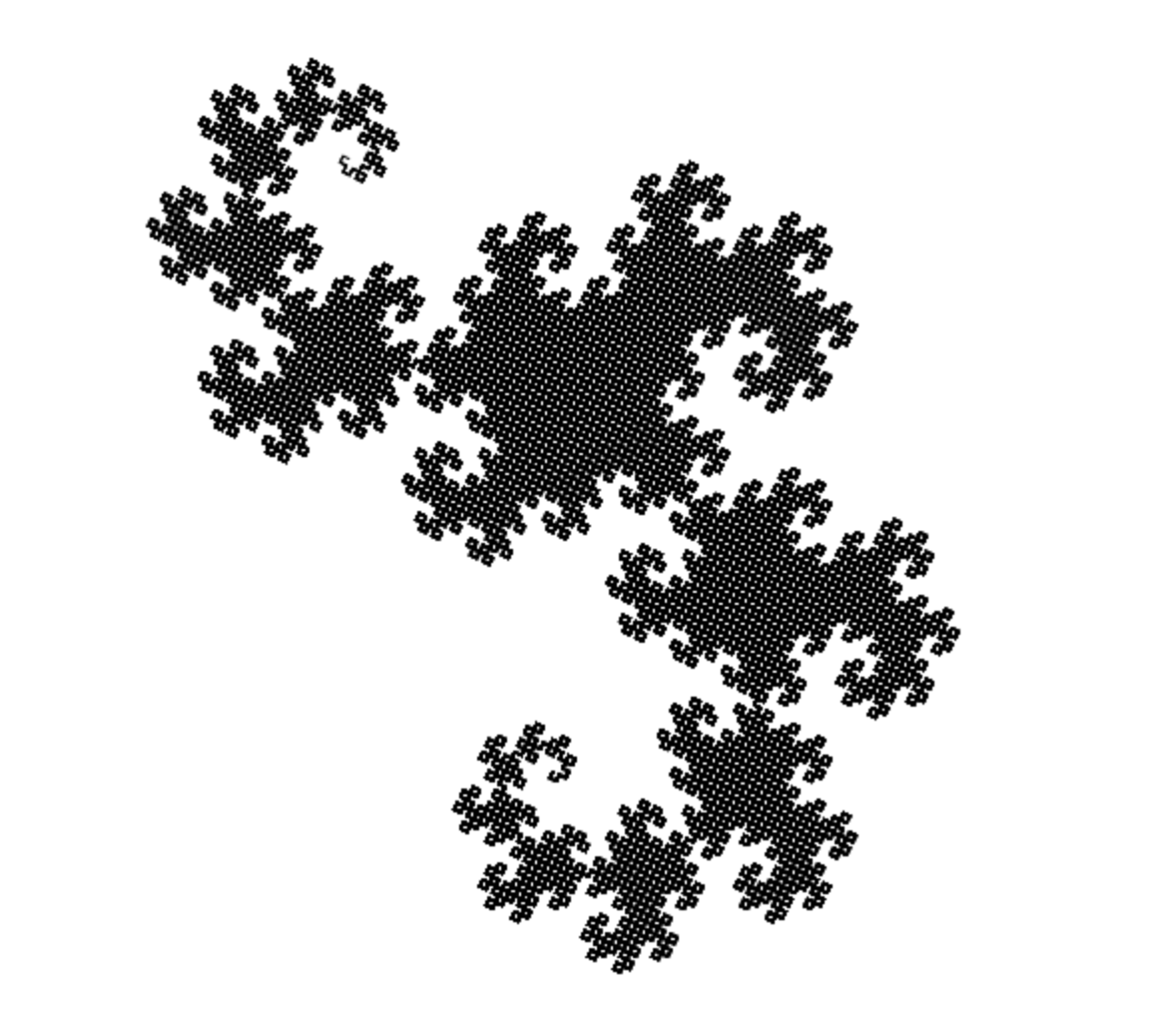
Dragon Fractal

**variables** : X Y
**constants** : F + −
**start** : FX
**rules** : (X → X+YF+), (Y → −FX−Y)
**angle** : 90°

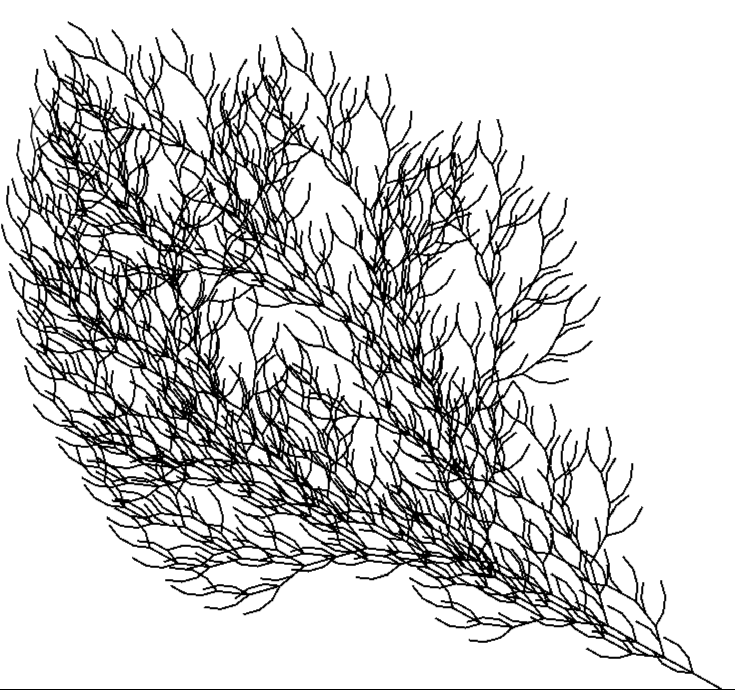
Fractal Curve Tree

**constants** : F + −
**start** : F
**rules** : F → FF-[-F+F+F]+[+F-F-F]
**angle** : 22.5°

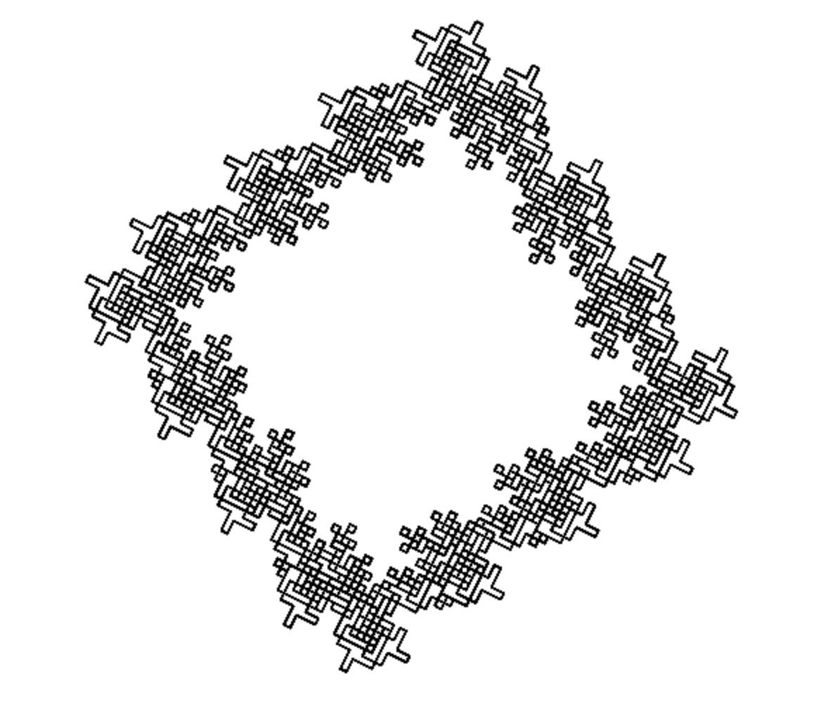
Closed Fractal

**variables** : X Y
**constants** : F + −
**start** : XYXYXYX+XYXYXYX+XYXYXYX+XYXYXYX
**rules** : (F → ), (X → FX+FX+FXFY-FY-) , (Y → +FX+FXFY-FY-FY)
**angle** : 90°

Code : https://github.com/Spockuto/LSystems

Live demo : http://vsekar.me/LSystems

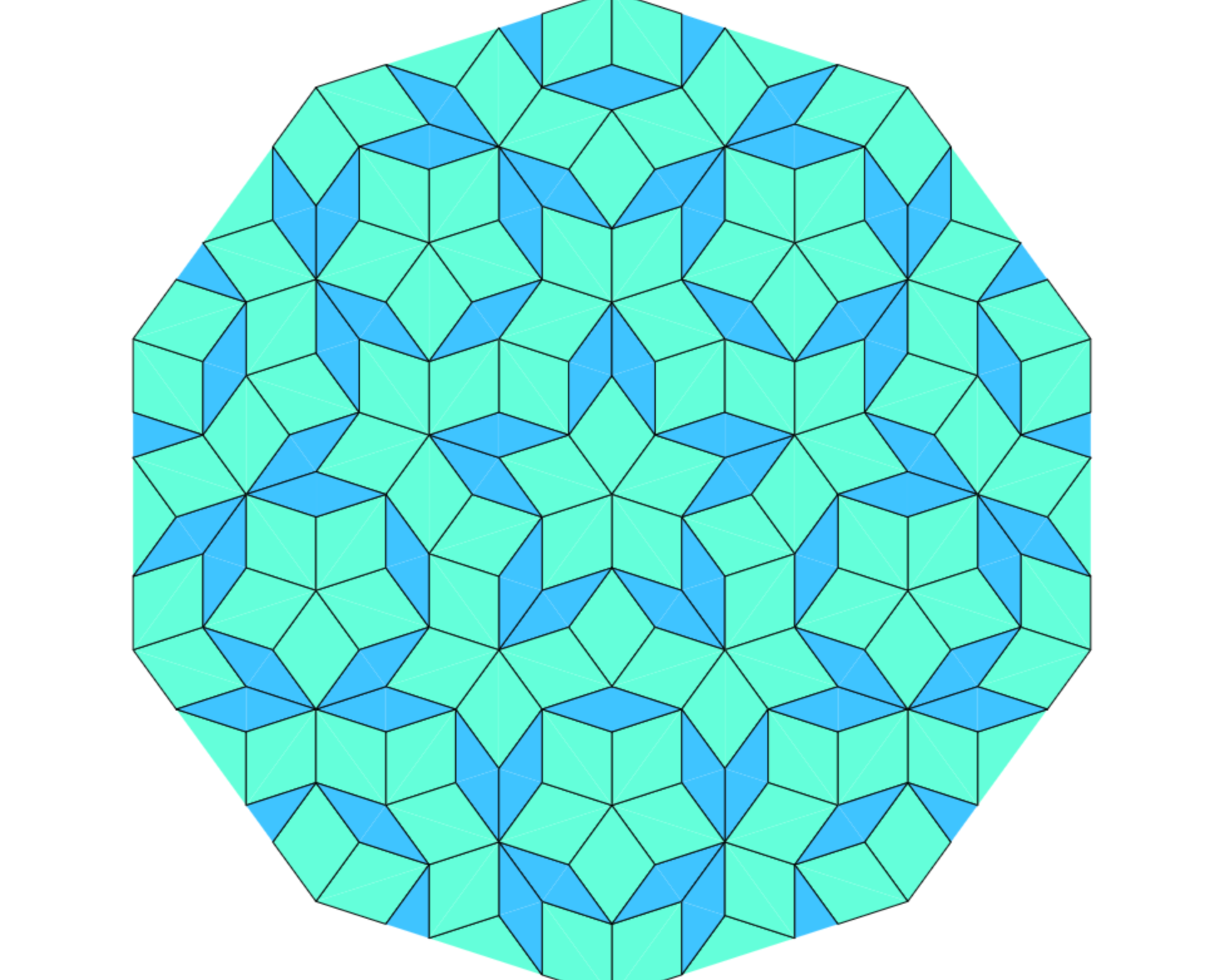
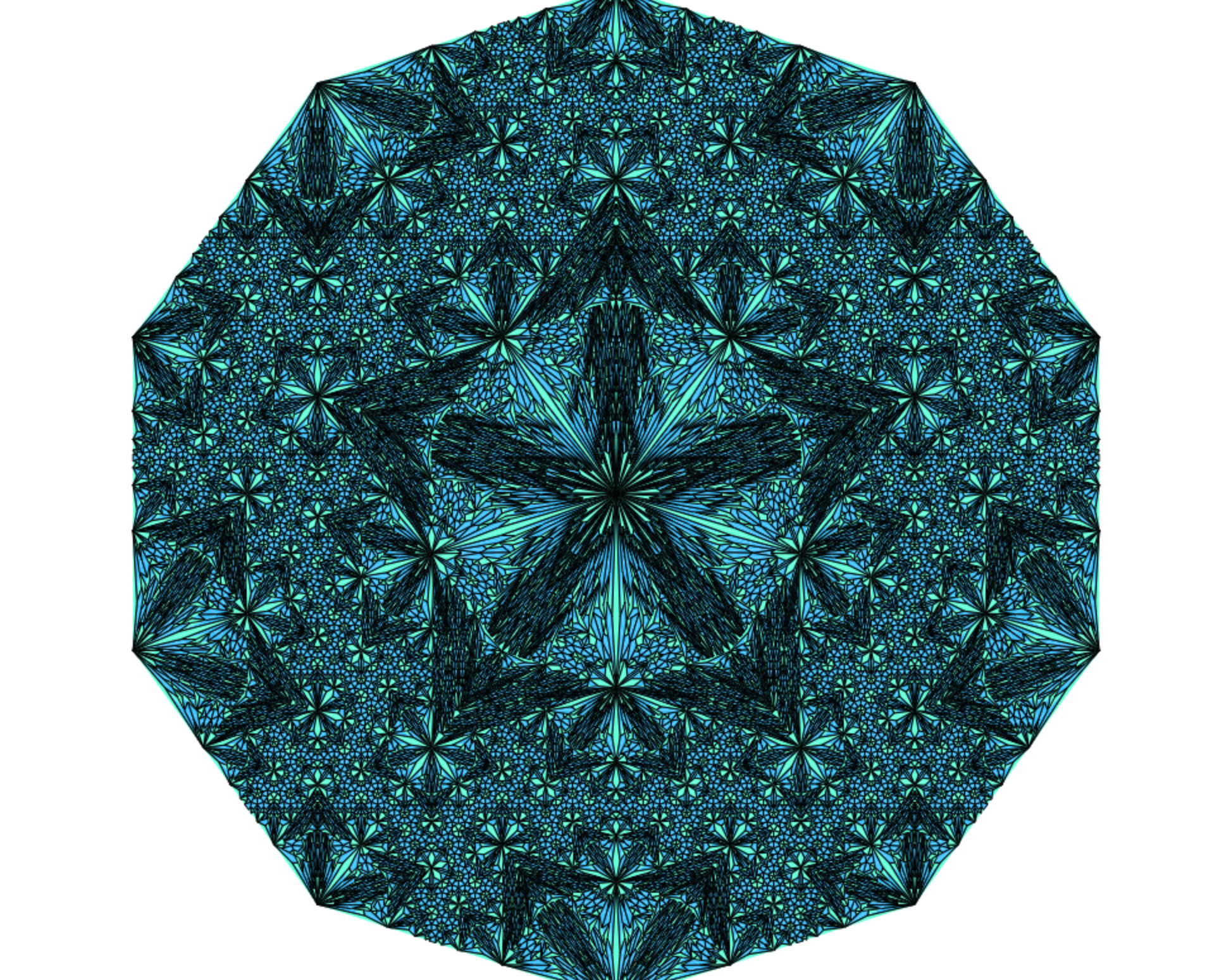
Penrose Tiling

Penrose tiling is a non-periodic tessellation generated by an aperiodic set of tiles. A tessellation of a flat surface is the tiling of a plane using one or more geometric shapes, called tiles, with no overlaps and no gaps. The aperiodicity of tiles implies that a shifted copy of a tiling will never match the original. It is self-similar, so the same patterns occur at larger and larger scales. Thus, the tiling can be obtained through “inflation” or “deflation” and every finite patch from the tiling occurs infinitely many times.

Penrose’s first tiling uses pentagons and three other shapes: a five-pointed “star” (a pentagram), a “boat” (roughly 3/5 of a star) and a “diamond” (a thin rhombus). Penrose’s second tiling uses quadrilaterals called the “kite” and “dart”, which may be combined to make a rhombus. Penrose Tiling Explained

This article explains the basic algorithm behind the tiling. Several properties and common features of the Penrose tilings involve the golden ratio φ = (1+√5)/2 (approximately 1.618).

Code : https://github.com/Spockuto/Penrose

Live demo : http://vsekar.me/Penrose

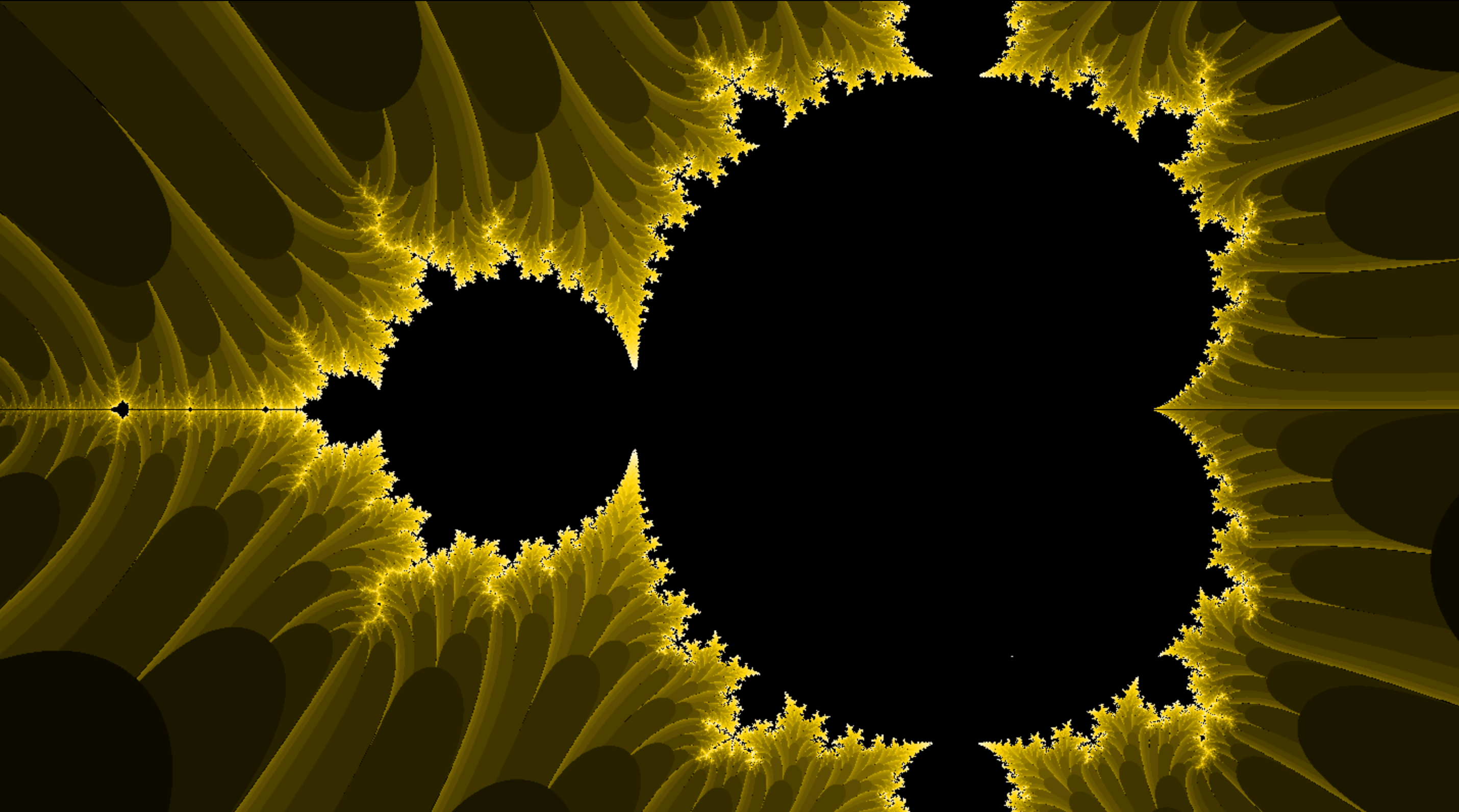
Mandlebrot Sets

It’s the the set of all complex numbers z for which the sequence defined by the iteration :

*z(0) = z,    z(n+1) = z(n)*z(n) + z,    n=0,1,2, ... *  

remains bounded. This means that there is a number ***B ***such that the absolute value of all iterates *z(n) *never gets larger than B. A bounded sequence may or not have a limit.

For example, if *z=0 *then z(n) = 0 for all n, so that the limit of the (1) is zero. On the other hand, if *z=i *( i being the imaginary unit), then the sequence oscillates between i and i-1, so remains bounded but it does not converge to a limit.

Treating the real and imaginary parts of *z *as image coordinates on the complex plane, pixels may then be coloured according to how soon the sequence crosses an arbitrarily chosen threshold, with a special colour (usually black) used for the values of *z *for which the sequence has not crossed the threshold after the predetermined number of iterations (this is necessary to clearly distinguish the Mandelbrot set image from the image of its complement).

**Images of the Mandelbrot set exhibit an elaborate and infinitely complicated boundary that reveals progressively ever-finer recursive detail at increasing magnifications. The “style” of this repeating detail depends on the region of the set being examined. The set’s boundary also incorporates smaller versions of the main shape, so the fractal property of self-similarity applies to the entire set, and not just to its parts.

Code : https://github.com/Spockuto/Mandelbrot

Live demo : https://vsekar.me/Mandelbrot/